This material is adapted from the article Microrobots and Micromechanical Systems by W. S. N. Trimmer, Sensors and Actuators, Volume 19, Number 3, September 1989, pages 267 - 287, and other sources. The book "Micromechanics and MEMS" has this and other interesting articles on small mechanical systems; published by the IEEE Press, number PC4390, ISBN 0-7803-1085-3. A more detailed analysis of the scaling of electromagnetic forces is given in the Appendix to Microrobots and Micromechanical Systems.A nice description of scaling is given in Trimmers Vertical Bracket Notation in the book Fundamentals of Microfabrication by Marc Madou, ISBN 0-8493-9451-1, CRC Press 1997.
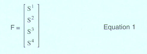
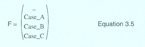
This paper uses a matrix formalism to describe the scaling
laws. This nomenclature shows a number of different force laws in a single
equation. In this notation, the size of the system is represented by a
single scale variable, S, which represents the linear scale of the system.
The choice of S for a system is a bit arbitrary. The S could be the separation
between the plates of a capacitor, or it could be the length of one edge
of the capacitor. Once chosen, however, it is assumed that all dimensions
of the system are equally scaled down in size as S is decreased (isometric
scaling). For example, nominally S = 1; if S is then changed to 0.1, all
the dimensions of the system are decreased by a factor of ten. A number
of different cases are shown in one equation. For example,
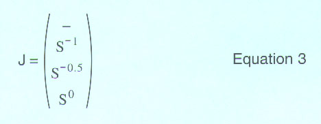
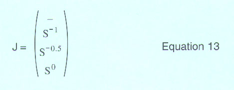
In summary, the currents required for the different force
laws scale as:
Electrostatic forces
Electrostatic actuators have a distinguished history,
but are not in general use for motors. (If you can, get a copy of
the delightful book by O. D. Jefimenko, "Electrostatic Motors," Published
by Electret Science Company, Star city, 1973. It is difficult to
find, but contains beautiful illustrations of early electrostatic motors.)
Electrostatic forces, however, become significant in the micro domain and
have numerous potential applications. The exact form of the scaling of
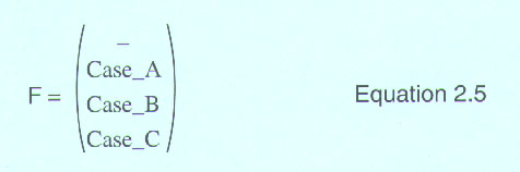
electrostatic forces depends upon how the E field changes with size. Generally,
the breakdown E field of insulators increases as the system becomes smaller.
Two cases will be examined here: (1) constant E field ( E= S0
); and (2) an E field that increases slightly as the system becomes smaller
(E = S-0.5 ). This second case exemplifies
the increasing E fields one can use as the system is scaled down.
(An early paper by Paschen discusses the increase in the breakdown
E field as a gap becomes smaller. F. Paschen, Uber die zum Funkenubergang
in Luft, Wasserstoff and Kohlensaure bei verschiedenen Drucken erforderliche
Potentialdifferenz. Annalen der Physick, 37:69-96, 1889. Also
Marc Madou's book "Fundamentals of Microfabrication" has a description
and plot of Paschen's curve on page 59.)
For the constant electric field ( E = S0 )
the force scales as S2 When E scales as S-0.5
, then the force has the even better scaling of F = S1
. When the size of the system is decreased, both of these force laws
give increasing accelerations and smaller transit times.
Other forces
There are several other interesting forces. Biological forces from muscle are proportional to the cross section of the muscle, and scale as S2 Pneumatic and hydraulic forces are caused by pressures (P) and also scale as S2. Large forces can be generated in the micro domain using pressure related forces. Surface tension has an absolutely delightful scaling of S1 , because it depends upon the length of the interface.
The unit cube
Below is a discussion of how the above force laws affect
the acceleration, transit time, power generation and power dissipation
as one scales to smaller domains. In going from here to there as quickly
as possible with a certain force, one wants to accelerate for half the
distance, and then decelerate. The mass of the object scales as S3
(density is assumed to be intensive, or to not change with scale). Now
the acceleration is given by equations of dynamics as:
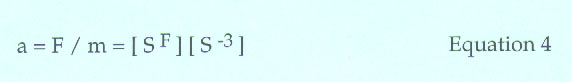
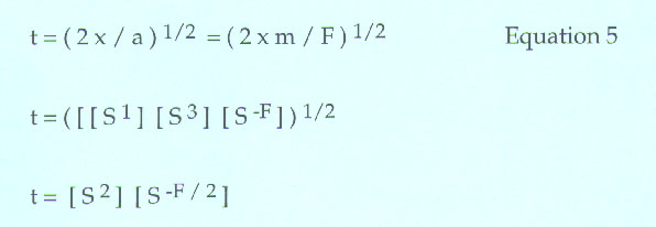
where SF represents the scaling
of the force F. Here only the time to accelerate has been calculated, but
an equal time is needed to decelerate, and both these times scale in the
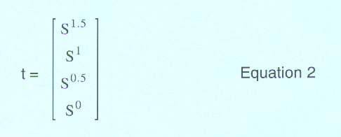
same way. For the forces given in equation (1), the accelerations and transit
times can be expressed as
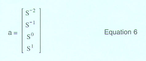
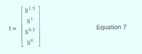
Even in the worst case, where F = S4
(the bottom element), the time required to perform a task remains
constant, t = S0 , when the system is scaled down. Under more
favorable force scaling, for example, the F = S2
scaling case, the time required decreases as t = S1 with
the scale. A system ten times smaller can perform an operation ten times
faster. This is an observation that we know intuitively: small things tend
to be quick.
Inertial forces tend to become insignificant in the small
domain, and in many cases kinematics may replace dynamics. This will probably
lead to interesting new control strategies.
Power generated and dissipated
As the scale of a system is changed, one wants to know
how the power produced depends upon the force laws. For example, consider
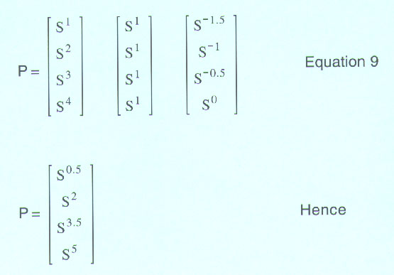
the unit cube above, which is first accelerated and then decelerated. The
power, P, or the work done on the object per unit time is
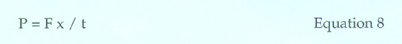
The scaling of each of the terms on the right is known.
The power that can be produced per unit volume ( V= S3 ) is
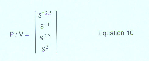
When the force scales as S2 then
the power per unit volume scales as S-1 . For example,
when the scale decreases by a factor of ten, the power that can be generated
per unit volume increases by a factor of ten. For force laws with a higher
power than S2 , the power generated per volume degrades
as the scale size decreases. There are several attractive force laws that
behave as S2, and one should try to use these forces
when designing small systems. (Please remember, these force laws depend
upon general assumptions, there is always room to be clever.)
For the magnetic case, one may be concerned about the
power dissipated by the resistive loss of the wires. The power due to this
resistive loss, PR, is
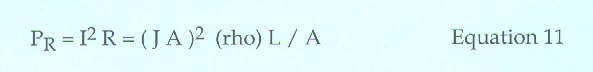
where A is the cross section of the wire, (rho) is the
resistivity of the wire, and L is the length of the wire. This gives
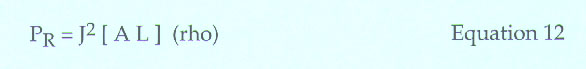
where (A L) is the volume. The resistivity scales as
S0 and the volume scales as S3
and from equation (3) above,
Hence the power dissipated scales as:
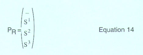
and the power per unit volume is:
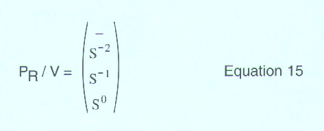
For the magnetic case A) where force scales as S2,
the power that must be dissipated per unit volume scales as S-2
, or, when the scale is decreased by a factor of ten, a hundred times as
much power must be dissipated within a set volume. This magnetic case is
bad if one is concerned about power density or the amount of cooling needed.
If power dissipation or cooling are not a critical concern, then this scaling
case produces more substantial forces. In the future, superconductors may
give us stronger micro electromagnets.
Summary of the scaling results
The force has been found to scale in one of four different ways: [ S1 ] , [ S2 ] , [ S3 ] , and [ S4 ] . If the scale size is decreased by a factor of ten, the forces for these different laws decrease by ten, one hundred, one thousand, and ten thousand respectively. In most cases, one wants to work with force laws that behave as [ S1 ] or [ S2 ] . The different cases that lead to these force laws, the accelerations, the transit times, and the power generated per unit volume are given below.
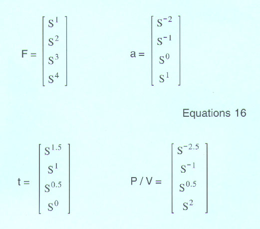
and
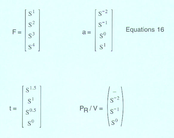
For the force laws that behave as [ S1 ] or
[ S2 ] , the acceleration increases as one scales down the system.
The power that can be produced per unit volume also increases for these
two laws. The surface tension scales advantageously, [ S1 ]
, however, it is not clear how to use this force in most applications.
Biological forces also scale well, [ S2 ] but may be difficult
to implement. Electrostatic and pressure related forces appear to be quite
useful forces in the small domain.